Information gain ratio

In decision tree learning, information gain ratio is a ratio of information gain to the intrinsic information. It was proposed by Ross Quinlan,^[1] to reduce a bias towards multi-valued attributes by taking the number and size of branches into account when choosing an attribute.^[2]

Information gain is also known as mutual information.^[3]

The image shows the information gain of a variable called "year" and shows the result of choosing a year 1 through 12. The information gain would favor this variable as the results would either be definitely positive or negative while also creating multiple leaf nodes, however, the problem is that none of these years will occur again. The next input would be year 13, but there is no branch to year 13 and that is a problem that can be solved with information gain ratio. Information gain ratio will normalize the data using the entropy value of that variable to remove the bias of multi-variable data and variables with multiple nodes compared to variables with a smaller set of nodes. This would remove the odds of the tree in the image from being created.

Information gain calculation

Information gain is the reduction in entropy produced from partitioning a set with attributes $a$ and finding the optimal candidate that produces the highest value:

{\text{IG}}(T,a)=\mathrm {H} {(T)}-\mathrm {H} {(T|a)},

where $T$ is a random variable and $\mathrm {H} {(T|a)}$ is the entropy of $T$ given the value of attribute $a$ .

The information gain is equal to the total entropy for an attribute if for each of the attribute values a unique classification can be made for the result attribute. In this case the relative entropies subtracted from the total entropy are 0.

Split information calculation

The split information value for a test is defined as follows:

${\text{SplitInformation}}(X)=-\sum _{i=1}^{n}{{\frac {\mathrm {N} (x_{i})}{\mathrm {N} (x)}}*\log {_{2}}{\frac {\mathrm {N} (x_{i})}{\mathrm {N} (x)}}}$

where $X$ is a discrete random variable with possible values ${x_{1},x_{2},...,x_{i}}$ and $N(x_{i})$ being the number of times that $x_{i}$ occurs divided by the total count of events $N(x)$ where $x$ is the set of events.

The split information value is a positive number that describes the potential worth of splitting a branch from a node. This in turn is the intrinsic value that the random variable possesses and will be used to remove the bias in the information gain ratio calculation.

Information gain ratio calculation

The information gain ratio is the ratio between the information gain and the split information value: ${\text{IGR}}(T,a)={\text{IG}}(T,a)/{\text{SplitInformation}}(T)$

${\text{IGR}}(T,a)={\frac {-\sum _{i=1}^{n}{\mathrm {P} (T)\log \mathrm {P} (T)}-(-\sum _{i=1}^{n}{\mathrm {P} (T|a)\log \mathrm {P} (T|a)})}{-\sum _{i=1}^{n}{{\frac {\mathrm {N} (t_{i})}{\mathrm {N} (t)}}*\log {_{2}}{\frac {\mathrm {N} (t_{i})}{\mathrm {N} (t)}}}}}$

Example

Using weather data published by Fordham University,^[4] the table was created below:

WEKA weather data
Outlook	Temperature	Humidity	Wind	Play
Sunny	Hot	High	False	No
Sunny	Hot	High	True	No
Overcast	Hot	High	False	Yes
Rainy	Mild	High	False	Yes
Rainy	Cool	Normal	False	Yes
Rainy	Cool	Normal	True	No
Overcast	Cool	Normal	True	Yes
Sunny	Mild	High	False	No
Sunny	Cool	Normal	False	Yes
Rainy	Mild	Normal	False	Yes
Sunny	Mild	Normal	False	Yes
Overcast	Mild	High	True	Yes
Overcast	Hot	Normal	False	Yes
Rainy	Mild	High	True	No

Using the table above, one can find the entropy, information gain, split information, and information gain ratio for each variable (outlook, temperature, humidity, and wind). These calculations are shown in the tables below:

Outlook table
Outlook	Yes	No	Count of each group	Entropy
sunny	2	3	5	0.971
overcast	4	0	4	0.000
rainy	3	2	5	0.971
Results	Values
Information	0.694
Overall entropy	0.940
Information gain	0.247
Split information	1.577
Gain ratio	0.156

Temperature table
Temperature	Yes	No	Count of each group	Entropy
hot	2	2	4	1.000
mild	4	2	6	0.918
cool	3	1	4	0.811
Results	Values
Information	0.911
Overall entropy	0.940
Information gain	0.029
Split information	1.557
Gain ratio	0.019

Wind table
Wind	Yes	No	Count of each group	Entropy
False	6	2	8	0.811
True	3	3	6	1.000
Results	Values
Information	0.892
Overall entropy	0.940
Information gain	0.048
Split information	0.985
Gain ratio	0.049

Humidity table
Humidity	Yes	No	Count of each group	Entropy
High	3	4	7	0.985
Normal	6	1	7	0.592
Results	Values
Information	0.788
Overall entropy	0.940
Information gain	0.152
Split information	1.000
Gain ratio	0.152

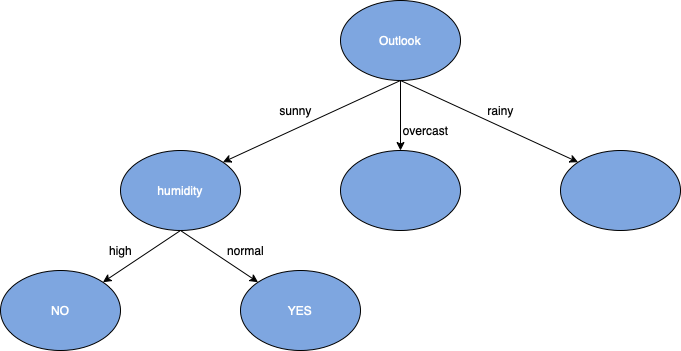
Using the above tables, one can deduce that Outlook has the highest information gain ratio. Next, one must find the statistics for the sub-groups of the Outlook variable (sunny, overcast, and rainy), for this example one will only build the sunny branch (as shown in the table below):

Outlook table
Outlook	Temperature	Humidity	Wind	Play
Sunny	Hot	High	False	No
Sunny	Hot	High	True	No
Sunny	Mild	High	False	No
Sunny	Cool	Normal	False	Yes
Sunny	Mild	Normal	True	Yes

One can find the following statistics for the other variables (temperature, humidity, and wind) to see which have the greatest effect on the sunny element of the outlook variable:

Temperature table
Temperature	Yes	No	Count of each group	Entropy
Hot	0	2	2	0.000
Mild	1	1	2	1.000
Cool	1	0	1	0.000
Results	Values
Information	0.400
Overall entropy	0.971
Gain	0.571
Split information	1.522
Gain ratio	0.375

Wind table
Wind	Yes	No	Count of each group	Entropy
False	1	2	3	0.918
True	1	1	2	1.000
Results	Values
Information	0.951
Overall entropy	0.971
Gain	0.020
Split information	0.971
Gain ratio	0.021

Humidity table
Humidity	Yes	No	Count of each group	Entropy
High	0	3	3	0.000
Normal	2	0	2	0.000
Results	Values
Information	0.000
Overall entropy	0.971
Gain	0.971
Split information	0.971
Gain ratio	1.000

Humidity was found to have the highest information gain ratio. One will repeat the same steps as before and find the statistics for the events of the Humidity variable (high and normal):

Humidity-high Table
Humidity	Wind	Play
High	False	No
High	True	No
High	False	No

Humidity-normal Table
Humidity	Wind	Play
Normal	False	Yes
Normal	True	Yes

Since the play values are either all "No" or "Yes", the information gain ratio value will be equal to 1. Also, now that one has reached the end of the variable chain with Wind being the last variable left, they can build an entire root to leaf node branch line of a decision tree.

Once finished with reaching this leaf node, one would follow the same procedure for the rest of the elements that have yet to be split in the decision tree. This set of data was relatively small, however, if a larger set was used, the advantages of using the information gain ratio as the splitting factor of a decision tree can be seen more.

Advantages

Information gain ratio biases the decision tree against considering attributes with a large number of distinct values.

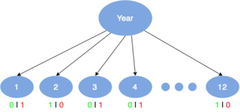
For example, suppose that we are building a decision tree for some data describing a business's customers. Information gain ratio is used to decide which of the attributes are the most relevant. These will be tested near the root of the tree. One of the input attributes might be the customer's telephone number. This attribute has a high information gain, because it uniquely identifies each customer. Due to its high amount of distinct values, this will not be chosen to be tested near the root.

Disadvantages

Although information gain ratio solves the key problem of information gain, it creates another problem. If one is considering an amount of attributes that have a high number of distinct values, these will never be above one that has a lower number of distinct values.

Difference from information gain

Information gain's shortcoming is created by not providing a numerical difference between attributes with high distinct values from those that have less.
- Example: Suppose that we are building a decision tree for some data describing a business's customers. Information gain is often used to decide which of the attributes are the most relevant, so they can be tested near the root of the tree. One of the input attributes might be the customer's credit card number. This attribute has a high information gain, because it uniquely identifies each customer, but we do not want to include it in the decision tree: deciding how to treat a customer based on their credit card number is unlikely to generalize to customers we haven't seen before.
Information gain ratio's strength is that it has a bias towards the attributes with the lower number of distinct values.
Below is a table describing the differences of information gain and information gain ratio when put in certain scenarios.

Situational differences between information gain and information gain ratio
Information gain	Information gain ratio
Will not favor any attributes by number of distinct values	Will favor attribute that have a lower number of distinct values
When applied to attributes that can take on a large number of distinct values, this technique might learn the training set too well	User will struggle if required to find attributes requiring a high number of distinct values

References

^ Quinlan, J. R. (1986). "Induction of decision trees". Machine Learning. 1: 81–106. doi:10.1007/BF00116251.
^ http://www.ke.tu-darmstadt.de/lehre/archiv/ws0809/mldm/dt.pdf Archived 2014-12-28 at the Wayback Machine ^{[bare URL PDF]}
^ "Information gain, mutual information and related measures".
^ https://storm.cis.fordham.edu/~gweiss/data-mining/weka-data/weather.nominal.arff

[1] Quinlan, J. R. (1986). "Induction of decision trees". Machine Learning. 1: 81–106. doi:10.1007/BF00116251.

[2] ttp://www.ke.tu-darmstadt.de/lehre/archiv/ws0809/mldm/dt.pdf Archived 2014-12-28 at the Wayback Machine ^{[bare URL PDF]}

[3] "Information gain, mutual information and related measures".

[4] ttps://storm.cis.fordham.edu/~gweiss/data-mining/weka-data/weather.nominal.arff

[1]

[2]

[3]

[4]

Fahrer / Team für die Suche eingeben: