In image processing, a kernel, convolution matrix, or mask is a small matrix used for blurring, sharpening, embossing, edge detection, and more. This is accomplished by doing a convolution between the kernel and an image. Or more simply, when each pixel in the output image is a function of the nearby pixels (including itself) in the input image, the kernel is that function.

The general expression of a convolution is

where is the filtered image, is the original image, is the filter kernel. Every element of the filter kernel is considered by and .

Depending on the element values, a kernel can cause a wide range of effects:

Operation	Kernel ω	Image result g(x,y)
Identity
Ridge or edge detection
Sharpen
Box blur (normalized)
Gaussian blur 3 × 3 (approximation)
Gaussian blur 5 × 5 (approximation)
Unsharp masking 5 × 5 Based on Gaussian blur with amount as 1 and threshold as 0 (with no image mask)

The above are just a few examples of effects achievable by convolving kernels and images.

The origin is the position of the kernel which is above (conceptually) the current output pixel. This could be outside of the actual kernel, though usually it corresponds to one of the kernel elements. For a symmetric kernel, the origin is usually the center element.

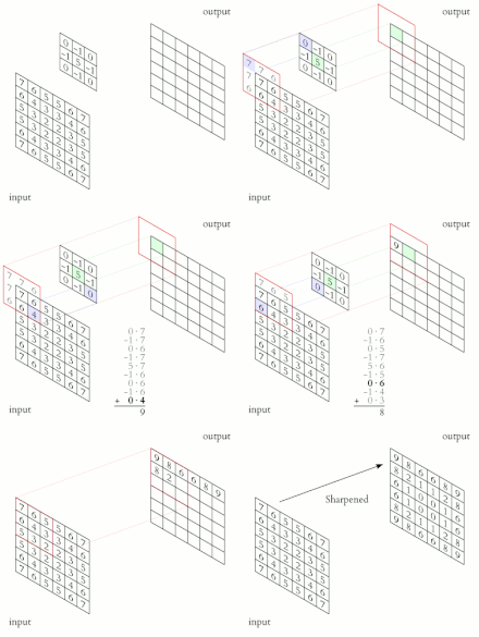
Convolution is the process of adding each element of the image to its local neighbors, weighted by the kernel. This is related to a form of mathematical convolution. The matrix operation being performed—convolution—is not traditional matrix multiplication, despite being similarly denoted by *.

For example, if we have two three-by-three matrices, the first a kernel, and the second an image piece, convolution is the process of flipping both the rows and columns of the kernel and multiplying locally similar entries and summing. The element at coordinates [2, 2] (that is, the central element) of the resulting image would be a weighted combination of all the entries of the image matrix, with weights given by the kernel:

The other entries would be similarly weighted, where we position the center of the kernel on each of the boundary points of the image, and compute a weighted sum.

The values of a given pixel in the output image are calculated by multiplying each kernel value by the corresponding input image pixel values. This can be described algorithmically with the following pseudo-code:

for each image row in input image:
    for each pixel in image row:

        set accumulator to zero

        for each kernel row in kernel:
            for each element in kernel row:

                if element position  corresponding* to pixel position then
                    multiply element value  corresponding* to pixel value
                    add result to accumulator
                endif

         set output image pixel to accumulator

*corresponding input image pixels are found relative to the kernel's origin.

If the kernel is symmetric then place the center (origin) of the kernel on the current pixel. The kernel will overlap the neighboring pixels around the origin. Each kernel element should be multiplied with the pixel value it overlaps with and all of the obtained values should be summed. This resultant sum will be the new value for the current pixel currently overlapped with the center of the kernel.

If the kernel is not symmetric, it has to be flipped both around its horizontal and vertical axis before calculating the convolution as above.^[1]

The general form for matrix convolution is

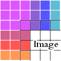
Kernel convolution usually requires values from pixels outside of the image boundaries. There are a variety of methods for handling image edges.

Extend

The nearest border pixels are conceptually extended as far as necessary to provide values for the convolution. Corner pixels are extended in 90° wedges. Other edge pixels are extended in lines.

Wrap

The image is conceptually wrapped (or tiled) and values are taken from the opposite edge or corner.

Mirror

The image is conceptually mirrored at the edges. For example, attempting to read a pixel 3 units outside an edge reads one 3 units inside the edge instead.

Crop / Avoid overlap

Any pixel in the output image which would require values from beyond the edge is skipped. This method can result in the output image being slightly smaller, with the edges having been cropped. Move kernel so that values from outside of image is never required. Machine learning mainly uses this approach. Example: Kernel size 10x10, image size 32x32, result image is 23x23.

Kernel Crop

Any pixel in the kernel that extends past the input image isn't used and the normalizing is adjusted to compensate.

Constant

Use constant value for pixels outside of image. Usually black or sometimes gray is used. Generally this depends on application.

Normalization is defined as the division of each element in the kernel by the sum of all kernel elements, so that the sum of the elements of a normalized kernel is unity. This will ensure the average pixel in the modified image is as bright as the average pixel in the original image.

Fast convolution algorithms include:

• separable convolution

2D convolution with an M × N kernel requires M × N multiplications for each sample (pixel). If the kernel is separable, then the computation can be reduced to M + N multiplications. Using separable convolutions can significantly decrease the computation by doing 1D convolution twice instead of one 2D convolution.^[2]

Here a concrete convolution implementation done with the GLSL shading language :

// author : csblo
// Work made just by consulting :
// https://en.wikipedia.org/wiki/Kernel_(image_processing)

// Define kernels
#define identity mat3(0, 0, 0, 0, 1, 0, 0, 0, 0)
#define edge0 mat3(1, 0, -1, 0, 0, 0, -1, 0, 1)
#define edge1 mat3(0, 1, 0, 1, -4, 1, 0, 1, 0)
#define edge2 mat3(-1, -1, -1, -1, 8, -1, -1, -1, -1)
#define sharpen mat3(0, -1, 0, -1, 5, -1, 0, -1, 0)
#define box_blur mat3(1, 1, 1, 1, 1, 1, 1, 1, 1) * 0.1111
#define gaussian_blur mat3(1, 2, 1, 2, 4, 2, 1, 2, 1) * 0.0625
#define emboss mat3(-2, -1, 0, -1, 1, 1, 0, 1, 2)

// Find coordinate of matrix element from index
vec2 kpos(int index)
{
    return vec2[9] (
        vec2(-1, -1), vec2(0, -1), vec2(1, -1),
        vec2(-1, 0), vec2(0, 0), vec2(1, 0), 
        vec2(-1, 1), vec2(0, 1), vec2(1, 1)
    )[index] / iResolution.xy;
}


// Extract region of dimension 3x3 from sampler centered in uv
// sampler : texture sampler
// uv : current coordinates on sampler
// return : an array of mat3, each index corresponding with a color channel
mat3[3] region3x3(sampler2D sampler, vec2 uv)
{
    // Create each pixels for region
    vec4[9] region;
    
    for (int i = 0; i < 9; i++)
        region[i] = texture(sampler, uv + kpos(i));

    // Create 3x3 region with 3 color channels (red, green, blue)
    mat3[3] mRegion;
    
    for (int i = 0; i < 3; i++)
        mRegion[i] = mat3(
        	region[0][i], region[1][i], region[2][i],
        	region[3][i], region[4][i], region[5][i],
        	region[6][i], region[7][i], region[8][i]
    	);
    
    return mRegion;
}

// Convolve a texture with kernel
// kernel : kernel used for convolution
// sampler : texture sampler
// uv : current coordinates on sampler
vec3 convolution(mat3 kernel, sampler2D sampler, vec2 uv)
{
    vec3 fragment;
    
    // Extract a 3x3 region centered in uv
    mat3[3] region = region3x3(sampler, uv);
    
    // for each color channel of region
    for (int i = 0; i < 3; i++)
    {
        // get region channel
        mat3 rc = region[i];
        // component wise multiplication of kernel by region channel
        mat3 c = matrixCompMult(kernel, rc);
        // add each component of matrix
        float r = c[0][0] + c[1][0] + c[2][0]
                + c[0][1] + c[1][1] + c[2][1]
                + c[0][2] + c[1][2] + c[2][2];
        
        // for fragment at channel i, set result
        fragment[i] = r;
    }
    
    return fragment;    
}

void mainImage( out vec4 fragColor, in vec2 fragCoord )
{
    // Normalized pixel coordinates (from 0 to 1)
    vec2 uv = fragCoord/iResolution.xy;
    // Convolve kernel with texture
    vec3 col = convolution(emboss, iChannel0, uv);
    
    // Output to screen
    fragColor = vec4(col, 1.0);
}

• Convolution in mathematics
• Multidimensional discrete convolution

• Ludwig, Jamie (n.d.). Image Convolution (PDF). Portland State University.
• Lecarme, Olivier; Delvare, Karine (January 2013). The Book of GIMP: A Complete Guide to Nearly Everything. No Starch Press. p. 429. ISBN 978-1593273835.
• Gumster, Jason van; Shimonski, Robert (March 2012). GIMP Bible. John Wiley & Sons. pp. 438–442. ISBN 978-0470523971.
• Shapiro, Linda G.; Stockman, George C. (February 2001). Computer Vision. Prentice Hall. pp. 53–54. ISBN 978-0130307965.

• Implementing 2d convolution on FPGA
• vImage Programming Guide: Performing Convolution Operations
• Image Processing using 2D-Convolution
• GNU Image Manipulation Program - User Manual - 8.2. Convolution Matrix
• GLSL Demonstration of 3x3 Convolution Kernels
• Complete C++ open source project

References

- ^ "Example of 2D Convolution".
- ^ "Convolution". www.songho.ca. Retrieved 2022-11-19.