Feedforward neural network
| Part of a series on |
| Machine learning and data mining |
|---|

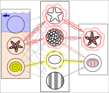
In reality, textures and outlines would not be represented by single nodes, but rather by associated weight patterns of multiple nodes.
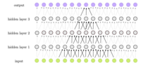
Feedforward refers to recognition-inference architecture of neural networks. Artificial neural network architectures are based on inputs multiplied by weights to obtain outputs (inputs-to-output): feedforward.[2] Recurrent neural networks, or neural networks with loops allow information from later processing stages to feed back to earlier stages for sequence processing.[3] However, at every stage of inference a feedforward multiplication remains the core, essential for backpropagation[4][5][6][7][8] or backpropagation through time. Thus neural networks cannot contain feedback like negative feedback or positive feedback where the outputs feed back to the very same inputs and modify them, because this forms an infinite loop which is not possible to rewind in time to generate an error signal through backpropagation. This issue and nomenclature appear to be a point of confusion between some computer scientists and scientists in other fields studying brain networks.[9]
Mathematical foundations
Activation function
The two historically common activation functions are both sigmoids, and are described by
- .
The first is a hyperbolic tangent that ranges from -1 to 1, while the other is the logistic function, which is similar in shape but ranges from 0 to 1. Here is the output of the th node (neuron) and is the weighted sum of the input connections. Alternative activation functions have been proposed, including the rectifier and softplus functions. More specialized activation functions include radial basis functions (used in radial basis networks, another class of supervised neural network models).
In recent developments of deep learning the rectified linear unit (ReLU) is more frequently used as one of the possible ways to overcome the numerical problems related to the sigmoids.
Learning
Learning occurs by changing connection weights after each piece of data is processed, based on the amount of error in the output compared to the expected result. This is an example of supervised learning, and is carried out through backpropagation.
We can represent the degree of error in an output node in the th data point (training example) by , where is the desired target value for th data point at node , and is the value produced at node when the th data point is given as an input.
The node weights can then be adjusted based on corrections that minimize the error in the entire output for the th data point, given by
- .
Using gradient descent, the change in each weight is
where is the output of the previous neuron , and is the learning rate, which is selected to ensure that the weights quickly converge to a response, without oscillations. In the previous expression, denotes the partial derivate of the error according to the weighted sum of the input connections of neuron .
The derivative to be calculated depends on the induced local field , which itself varies. It is easy to prove that for an output node this derivative can be simplified to
where is the derivative of the activation function described above, which itself does not vary. The analysis is more difficult for the change in weights to a hidden node, but it can be shown that the relevant derivative is
- .
This depends on the change in weights of the th nodes, which represent the output layer. So to change the hidden layer weights, the output layer weights change according to the derivative of the activation function, and so this algorithm represents a backpropagation of the activation function.[10]
History
Timeline
- Circa 1800, Legendre (1805) and Gauss (1795) created the simplest feedforward network which consists of a single weight layer with linear activation functions. It was trained by the least squares method for minimising mean squared error, also known as linear regression. Legendre and Gauss used it for the prediction of planetary movement from training data.[11][12][13][14][15]
- In 1943, Warren McCulloch and Walter Pitts proposed the binary artificial neuron as a logical model of biological neural networks.[16]
- In 1958, Frank Rosenblatt proposed the multilayered perceptron model, consisting of an input layer, a hidden layer with randomized weights that did not learn, and an output layer with learnable connections.[17] R. D. Joseph (1960)[18] mentions an even earlier perceptron-like device:[13] "Farley and Clark of MIT Lincoln Laboratory actually preceded Rosenblatt in the development of a perceptron-like device." However, "they dropped the subject."
- In 1960, Joseph[18] also discussed multilayer perceptrons with an adaptive hidden layer. Rosenblatt (1962)[19]: section 16 cited and adopted these ideas, also crediting work by H. D. Block and B. W. Knight. Unfortunately, these early efforts did not lead to a working learning algorithm for hidden units, i.e., deep learning.
- In 1965, Alexey Grigorevich Ivakhnenko and Valentin Lapa published Group Method of Data Handling, the first working deep learning algorithm, a method to train arbitrarily deep neural networks.[20][21] It is based on layer by layer training through regression analysis. Superfluous hidden units are pruned using a separate validation set. Since the activation functions of the nodes are Kolmogorov-Gabor polynomials, these were also the first deep networks with multiplicative units or "gates."[13] It was used to train an eight-layer neural net in 1971.
- In 1967, Shun'ichi Amari reported [22] the first multilayered neural network trained by stochastic gradient descent, which was able to classify non-linearily separable pattern classes. Amari's student Saito conducted the computer experiments, using a five-layered feedforward network with two learning layers.[13]
- In 1970, Seppo Linnainmaa published the modern form of backpropagation in his master thesis (1970).[23][24][13] G.M. Ostrovski et al. republished it in 1971.[25][26] Paul Werbos applied backpropagation to neural networks in 1982[7][27] (his 1974 PhD thesis, reprinted in a 1994 book,[28] did not yet describe the algorithm[26]). In 1986, David E. Rumelhart et al. popularised backpropagation but did not cite the original work.[29][8]
- In 2003, interest in backpropagation networks returned due to the successes of deep learning being applied to language modelling by Yoshua Bengio with co-authors.[30]
Linear regression
Perceptron
If using a threshold, i.e. a linear activation function, the resulting linear threshold unit is called a perceptron. (Often the term is used to denote just one of these units.) Multiple parallel non-linear units are able to approximate any continuous function from a compact interval of the real numbers into the interval [−1,1] despite the limited computational power of single unit with a linear threshold function.[31]
Perceptrons can be trained by a simple learning algorithm that is usually called the delta rule. It calculates the errors between calculated output and sample output data, and uses this to create an adjustment to the weights, thus implementing a form of gradient descent.
Multilayer perceptron

A multilayer perceptron (MLP) is a misnomer for a modern feedforward artificial neural network, consisting of fully connected neurons (hence the synonym sometimes used of fully connected network (FCN)), often with a nonlinear kind of activation function, organized in at least three layers, notable for being able to distinguish data that is not linearly separable.[32]
Other feedforward networks

Examples of other feedforward networks include convolutional neural networks and radial basis function networks, which use a different activation function.
See also
References
- ^ Ferrie, C., & Kaiser, S. (2019). Neural Networks for Babies. Sourcebooks. ISBN 978-1492671206.
{{cite book}}: CS1 maint: multiple names: authors list (link) - ^ Zell, Andreas (1994). Simulation Neuronaler Netze [Simulation of Neural Networks] (in German) (1st ed.). Addison-Wesley. p. 73. ISBN 3-89319-554-8.
- ^ Schmidhuber, Jürgen (2015-01-01). "Deep learning in neural networks: An overview". Neural Networks. 61: 85–117. arXiv:1404.7828. doi:10.1016/j.neunet.2014.09.003. ISSN 0893-6080. PMID 25462637. S2CID 11715509.
- ^ Linnainmaa, Seppo (1970). The representation of the cumulative rounding error of an algorithm as a Taylor expansion of the local rounding errors (Masters) (in Finnish). University of Helsinki. p. 6–7.
- ^ Kelley, Henry J. (1960). "Gradient theory of optimal flight paths". ARS Journal. 30 (10): 947–954. doi:10.2514/8.5282.
- ^ Rosenblatt, Frank. x. Principles of Neurodynamics: Perceptrons and the Theory of Brain Mechanisms. Spartan Books, Washington DC, 1961
- ^ a b Werbos, Paul (1982). "Applications of advances in nonlinear sensitivity analysis" (PDF). System modeling and optimization. Springer. pp. 762–770. Archived (PDF) from the original on 14 April 2016. Retrieved 2 July 2017.
- ^ a b Rumelhart, David E., Geoffrey E. Hinton, and R. J. Williams. "Learning Internal Representations by Error Propagation". David E. Rumelhart, James L. McClelland, and the PDP research group. (editors), Parallel distributed processing: Explorations in the microstructure of cognition, Volume 1: Foundation. MIT Press, 1986.
- ^ Achler, T. (2023). "What AI, Neuroscience, and Cognitive Science Can Learn from Each Other: An Embedded Perspective". Cognitive Computation.
- ^ Haykin, Simon (1998). Neural Networks: A Comprehensive Foundation (2 ed.). Prentice Hall. ISBN 0-13-273350-1.
- ^ Merriman, Mansfield. A List of Writings Relating to the Method of Least Squares: With Historical and Critical Notes. Vol. 4. Academy, 1877.
- ^ Stigler, Stephen M. (1981). "Gauss and the Invention of Least Squares". Ann. Stat. 9 (3): 465–474. doi:10.1214/aos/1176345451.
- ^ a b c d e Schmidhuber, Jürgen (2022). "Annotated History of Modern AI and Deep Learning". arXiv:2212.11279 [cs.NE].
- ^ Bretscher, Otto (1995). Linear Algebra With Applications (3rd ed.). Upper Saddle River, NJ: Prentice Hall.
- ^ Stigler, Stephen M. (1986). The History of Statistics: The Measurement of Uncertainty before 1900. Cambridge: Harvard. ISBN 0-674-40340-1.
- ^ McCulloch, Warren S.; Pitts, Walter (1943-12-01). "A logical calculus of the ideas immanent in nervous activity". The Bulletin of Mathematical Biophysics. 5 (4): 115–133. doi:10.1007/BF02478259. ISSN 1522-9602.
- ^ Rosenblatt, Frank (1958). "The Perceptron: A Probabilistic Model For Information Storage And Organization in the Brain". Psychological Review. 65 (6): 386–408. CiteSeerX 10.1.1.588.3775. doi:10.1037/h0042519. PMID 13602029. S2CID 12781225.
- ^ a b Joseph, R. D. (1960). Contributions to Perceptron Theory, Cornell Aeronautical Laboratory Report No. VG-11 96--G-7, Buffalo.
- ^ Rosenblatt, Frank (1962). Principles of Neurodynamics. Spartan, New York.
- ^ Ivakhnenko, A. G. (1973). Cybernetic Predicting Devices. CCM Information Corporation.
- ^ Ivakhnenko, A. G.; Grigorʹevich Lapa, Valentin (1967). Cybernetics and forecasting techniques. American Elsevier Pub. Co.
- ^ Amari, Shun'ichi (1967). "A theory of adaptive pattern classifier". IEEE Transactions. EC (16): 279-307.
- ^ Linnainmaa, Seppo (1970). The representation of the cumulative rounding error of an algorithm as a Taylor expansion of the local rounding errors (Masters) (in Finnish). University of Helsinki. p. 6–7.
- ^ Linnainmaa, Seppo (1976). "Taylor expansion of the accumulated rounding error". BIT Numerical Mathematics. 16 (2): 146–160. doi:10.1007/bf01931367. S2CID 122357351.
- ^ Ostrovski, G.M., Volin,Y.M., and Boris, W.W. (1971). On the computation of derivatives. Wiss. Z. Tech. Hochschule for Chemistry, 13:382–384.
- ^ a b Schmidhuber, Juergen (25 Oct 2014). "Who Invented Backpropagation?". IDSIA, Switzerland. Archived from the original on 30 July 2024. Retrieved 14 Sep 2024.
- ^ Anderson, James A.; Rosenfeld, Edward, eds. (2000). Talking Nets: An Oral History of Neural Networks. The MIT Press. doi:10.7551/mitpress/6626.003.0016. ISBN 978-0-262-26715-1.
- ^ Werbos, Paul J. (1994). The Roots of Backpropagation : From Ordered Derivatives to Neural Networks and Political Forecasting. New York: John Wiley & Sons. ISBN 0-471-59897-6.
- ^ Rumelhart, David E.; Hinton, Geoffrey E.; Williams, Ronald J. (October 1986). "Learning representations by back-propagating errors". Nature. 323 (6088): 533–536. Bibcode:1986Natur.323..533R. doi:10.1038/323533a0. ISSN 1476-4687.
- ^ Bengio, Yoshua; Ducharme, Réjean; Vincent, Pascal; Janvin, Christian (March 2003). "A neural probabilistic language model". The Journal of Machine Learning Research. 3: 1137–1155.
- ^ Auer, Peter; Harald Burgsteiner; Wolfgang Maass (2008). "A learning rule for very simple universal approximators consisting of a single layer of perceptrons" (PDF). Neural Networks. 21 (5): 786–795. doi:10.1016/j.neunet.2007.12.036. PMID 18249524. Archived from the original (PDF) on 2011-07-06. Retrieved 2009-09-08.
- ^ Cybenko, G. 1989. Approximation by superpositions of a sigmoidal function Mathematics of Control, Signals, and Systems, 2(4), 303–314.


