Smith–Waterman algorithm
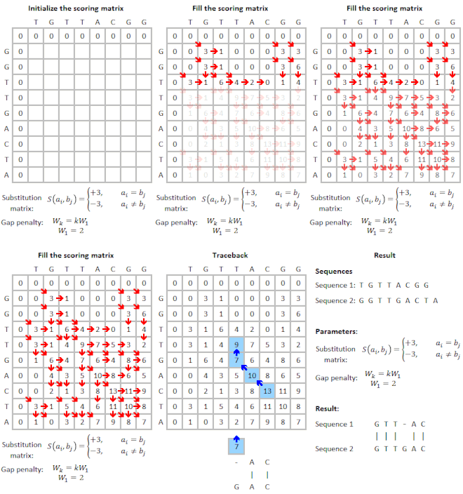 An animated example to show the steps progressively. See here for detailed steps. | |
| Class | Sequence alignment |
|---|---|
| Worst-case performance | |
| Worst-case space complexity | |
The Smith–Waterman algorithm performs local sequence alignment; that is, for determining similar regions between two strings of nucleic acid sequences or protein sequences. Instead of looking at the entire sequence, the Smith–Waterman algorithm compares segments of all possible lengths and optimizes the similarity measure.
The algorithm was first proposed by Temple F. Smith and Michael S. Waterman in 1981.[1] Like the Needleman–Wunsch algorithm, of which it is a variation, Smith–Waterman is a dynamic programming algorithm. As such, it has the desirable property that it is guaranteed to find the optimal local alignment with respect to the scoring system being used (which includes the substitution matrix and the gap-scoring scheme). The main difference to the Needleman–Wunsch algorithm is that negative scoring matrix cells are set to zero. Traceback procedure starts at the highest scoring matrix cell and proceeds until a cell with score zero is encountered, yielding the highest scoring local alignment. Because of its cubic time complexity, it often cannot be practically applied to large-scale problems and is replaced in favor of computationally more efficient alternatives such as (Gotoh, 1982),[2] (Altschul and Erickson, 1986),[3] and (Myers and Miller, 1988).[4]
History
In 1970, Saul B. Needleman and Christian D. Wunsch proposed a heuristic homology algorithm for sequence alignment, also referred to as the Needleman–Wunsch algorithm.[5] It is a global alignment algorithm that requires calculation steps ( and are the lengths of the two sequences being aligned). It uses the iterative calculation of a matrix for the purpose of showing global alignment. In the following decade, Sankoff,[6] Reichert,[7] Beyer[8] and others formulated alternative heuristic algorithms for analyzing gene sequences. Sellers introduced a system for measuring sequence distances.[9] In 1976, Waterman et al. added the concept of gaps into the original measurement system.[10] In 1981, Smith and Waterman published their Smith–Waterman algorithm for calculating local alignment.
The Smith–Waterman algorithm is fairly demanding of time: To align two sequences of lengths and , time is required. Gotoh[2] and Altschul[3] optimized the algorithm to steps. The space complexity was optimized by Myers and Miller[4] from to (linear), where is the length of the shorter sequence, for the case where only one of the many possible optimal alignments is desired. Chowdhury, Le, and Ramachandran[11] later optimized the cache performance of the algorithm while keeping the space usage linear in the total length of the input sequences.
Motivation
In recent years, genome projects conducted on a variety of organisms generated massive amounts of sequence data for genes and proteins, which requires computational analysis. Sequence alignment shows the relations between genes or between proteins, leading to a better understanding of their homology and functionality. Sequence alignment can also reveal conserved domains and motifs.
One motivation for local alignment is the difficulty of obtaining correct alignments in regions of low similarity between distantly related biological sequences, because mutations have added too much 'noise' over evolutionary time to allow for a meaningful comparison of those regions. Local alignment avoids such regions altogether and focuses on those with a positive score, i.e. those with an evolutionarily conserved signal of similarity. A prerequisite for local alignment is a negative expectation score. The expectation score is defined as the average score that the scoring system (substitution matrix and gap penalties) would yield for a random sequence.
Another motivation for using local alignments is that there is a reliable statistical model (developed by Karlin and Altschul) for optimal local alignments. The alignment of unrelated sequences tends to produce optimal local alignment scores which follow an extreme value distribution. This property allows programs to produce an expectation value for the optimal local alignment of two sequences, which is a measure of how often two unrelated sequences would produce an optimal local alignment whose score is greater than or equal to the observed score. Very low expectation values indicate that the two sequences in question might be homologous, meaning they might share a common ancestor.
Algorithm
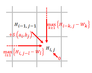
Let and be the sequences to be aligned, where and are the lengths of and respectively.
- Determine the substitution matrix and the gap penalty scheme.
- - Similarity score of the elements that constituted the two sequences
- - The penalty of a gap that has length
- Construct a scoring matrix and initialize its first row and first column. The size of the scoring matrix is . The matrix uses 0-based indexing.
- Fill the scoring matrix using the equation below.
- where
- is the score of aligning and ,
- is the score if is at the end of a gap of length ,
- is the score if is at the end of a gap of length ,
- means there is no similarity up to and .
- Traceback. Starting at the highest score in the scoring matrix and ending at a matrix cell that has a score of 0, traceback based on the source of each score recursively to generate the best local alignment.
Explanation
Smith–Waterman algorithm aligns two sequences by matches/mismatches (also known as substitutions), insertions, and deletions. Both insertions and deletions are the operations that introduce gaps, which are represented by dashes. The Smith–Waterman algorithm has several steps:
- Determine the substitution matrix and the gap penalty scheme. A substitution matrix assigns each pair of bases or amino acids a score for match or mismatch. Usually matches get positive scores, whereas mismatches get relatively lower scores. A gap penalty function determines the score cost for opening or extending gaps. It is suggested that users choose the appropriate scoring system based on the goals. In addition, it is also a good practice to try different combinations of substitution matrices and gap penalties.
- Initialize the scoring matrix. The dimensions of the scoring matrix are 1+length of each sequence respectively. All the elements of the first row and the first column are set to 0. The extra first row and first column make it possible to align one sequence to another at any position, and setting them to 0 makes the terminal gap free from penalty.
- Scoring. Score each element from left to right, top to bottom in the matrix, considering the outcomes of substitutions (diagonal scores) or adding gaps (horizontal and vertical scores). If none of the scores are positive, this element gets a 0. Otherwise the highest score is used and the source of that score is recorded.
- Traceback. Starting at the element with the highest score, traceback based on the source of each score recursively, until 0 is encountered. The segments that have the highest similarity score based on the given scoring system is generated in this process. To obtain the second best local alignment, apply the traceback process starting at the second highest score outside the trace of the best alignment.
Comparison with the Needleman–Wunsch algorithm
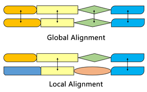
The Smith–Waterman algorithm finds the segments in two sequences that have similarities while the Needleman–Wunsch algorithm aligns two complete sequences. Therefore, they serve different purposes. Both algorithms use the concepts of a substitution matrix, a gap penalty function, a scoring matrix, and a traceback process. Three main differences are:
| Smith–Waterman algorithm | Needleman–Wunsch algorithm | |
|---|---|---|
| Initialization | First row and first column are set to 0 | First row and first column are subject to gap penalty |
| Scoring | Negative score is set to 0 | Score can be negative |
| Traceback | Begin with the highest score, end when 0 is encountered | Begin with the cell at the lower right of the matrix, end at top left cell |
One of the most important distinctions is that no negative score is assigned in the scoring system of the Smith–Waterman algorithm, which enables local alignment. When any element has a score lower than zero, it means that the sequences up to this position have no similarities; this element will then be set to zero to eliminate influence from previous alignment. In this way, calculation can continue to find alignment in any position afterwards.
The initial scoring matrix of Smith–Waterman algorithm enables the alignment of any segment of one sequence to an arbitrary position in the other sequence. In Needleman–Wunsch algorithm, however, end gap penalty also needs to be considered in order to align the full sequences.
Substitution matrix
Each base substitution or amino acid substitution is assigned a score. In general, matches are assigned positive scores, and mismatches are assigned relatively lower scores. Take DNA sequence as an example. If matches get +1, mismatches get -1, then the substitution matrix is:
| A | G | C | T | |
|---|---|---|---|---|
| A | 1 | -1 | -1 | -1 |
| G | -1 | 1 | -1 | -1 |
| C | -1 | -1 | 1 | -1 |
| T | -1 | -1 | -1 | 1 |
This substitution matrix can be described as:
Different base substitutions or amino acid substitutions can have different scores. The substitution matrix of amino acids is usually more complicated than that of the bases. See PAM, BLOSUM.
Gap penalty
Gap penalty designates scores for insertion or deletion. A simple gap penalty strategy is to use fixed score for each gap. In biology, however, the score needs to be counted differently for practical reasons. On one hand, partial similarity between two sequences is a common phenomenon; on the other hand, a single gene mutation event can result in insertion of a single long gap. Therefore, connected gaps forming a long gap usually is more favored than multiple scattered, short gaps. In order to take this difference into consideration, the concepts of gap opening and gap extension have been added to the scoring system. The gap opening score is usually higher than the gap extension score. For instance, the default parameters in EMBOSS Water are: gap opening = 10, gap extension = 0.5.
Here we discuss two common strategies for gap penalty. See Gap penalty for more strategies. Let be the gap penalty function for a gap of length :
Linear
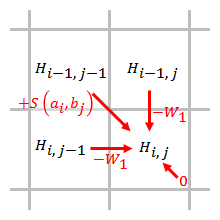
A linear gap penalty has the same scores for opening and extending a gap:
,
where is the cost of a single gap.
The gap penalty is directly proportional to the gap length. When linear gap penalty is used, the Smith–Waterman algorithm can be simplified to:
The simplified algorithm uses steps. When an element is being scored, only the gap penalties from the elements that are directly adjacent to this element need to be considered.
Affine
An affine gap penalty considers gap opening and extension separately:
,
where is the gap opening penalty, and is the gap extension penalty. For example, the penalty for a gap of length 2 is .
An arbitrary gap penalty was used in the original Smith–Waterman algorithm paper. It uses steps, therefore is quite demanding of time. Gotoh optimized the steps for an affine gap penalty to ,[2] but the optimized algorithm only attempts to find one optimal alignment, and the optimal alignment is not guaranteed to be found.[3] Altschul modified Gotoh's algorithm to find all optimal alignments while maintaining the computational complexity.[3] Later, Myers and Miller pointed out that Gotoh and Altschul's algorithm can be further modified based on the method that was published by Hirschberg in 1975,[12] and applied this method.[4] Myers and Miller's algorithm can align two sequences using space, with being the length of the shorter sequence. Chowdhury, Le, and Ramachandran[11] later showed how to run Gotoh's algorithm cache-efficiently in linear space using a different recursive divide-and-conquer strategy than the one used by Hirschberg. The resulting algorithm runs faster than Myers and Miller's algorithm in practice due to its superior cache performance.[11]
Gap penalty example
Take the alignment of sequences TACGGGCCCGCTAC and TAGCCCTATCGGTCA as an example. When linear gap penalty function is used, the result is (Alignments performed by EMBOSS Water. Substitution matrix is DNAfull (similarity score: +5 for matching characters otherwise -4). Gap opening and extension are 0.0 and 1.0 respectively):
TACGGGCCCGCTA-C

TA---G-CC-CTATC
When affine gap penalty is used, the result is (Gap opening and extension are 5.0 and 1.0 respectively):
TACGGGCCCGCTA

TA---GCC--CTA
This example shows that an affine gap penalty can help avoid scattered small gaps.
Scoring matrix
The function of the scoring matrix is to conduct one-to-one comparisons between all components in two sequences and record the optimal alignment results. The scoring process reflects the concept of dynamic programming. The final optimal alignment is found by iteratively expanding the growing optimal alignment. In other words, the current optimal alignment is generated by deciding which path (match/mismatch or inserting gap) gives the highest score from the previous optimal alignment. The size of the matrix is the length of one sequence plus 1 by the length of the other sequence plus 1. The additional first row and first column serve the purpose of aligning one sequence to any positions in the other sequence. Both the first line and the first column are set to 0 so that end gap is not penalized. The initial scoring matrix is:
| b1 | ... | bj | ... | bm | ||
|---|---|---|---|---|---|---|
| 0 | 0 | ... | 0 | ... | 0 | |
| a1 | 0 | |||||
| ... | ... | |||||
| ai | 0 | |||||
| ... | ... | |||||
| an | 0 |
Example
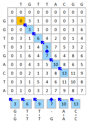
Take the alignment of DNA sequences TGTTACGG and GGTTGACTA as an example. Use the following scheme:
- Substitution matrix:
- Gap penalty: (a linear gap penalty of )
Initialize and fill the scoring matrix, shown as below. This figure shows the scoring process of the first three elements. The yellow color indicates the bases that are being considered. The red color indicates the highest possible score for the cell being scored.

The finished scoring matrix is shown below on the left. The blue color shows the highest score. An element can receive score from more than one element, each will form a different path if this element is traced back. In case of multiple highest scores, traceback should be done starting with each highest score. The traceback process is shown below on the right. The best local alignment is generated in the reverse direction.
 |
 |
| Finished scoring matrix (the highest score is in blue) | Traceback process and alignment result |
The alignment result is:
G T T - A C

G T T G A C
Implementation
An implementation of the Smith–Waterman Algorithm, SSEARCH, is available in the FASTA sequence analysis package from UVA FASTA Downloads. This implementation includes Altivec accelerated code for PowerPC G4 and G5 processors that speeds up comparisons 10–20-fold, using a modification of the Wozniak, 1997 approach,[13] and an SSE2 vectorization developed by Farrar[14] making optimal protein sequence database searches quite practical. A library, SSW, extends Farrar's implementation to return alignment information in addition to the optimal Smith–Waterman score.[15]
Accelerated versions
FPGA
Cray demonstrated acceleration of the Smith–Waterman algorithm using a reconfigurable computing platform based on FPGA chips, with results showing up to 28x speed-up over standard microprocessor-based solutions. Another FPGA-based version of the Smith–Waterman algorithm shows FPGA (Virtex-4) speedups up to 100x[16] over a 2.2 GHz Opteron processor.[17] The TimeLogic DeCypher and CodeQuest systems also accelerate Smith–Waterman and Framesearch using PCIe FPGA cards.
A 2011 Master's thesis [18] includes an analysis of FPGA-based Smith–Waterman acceleration.
In a 2016 publication OpenCL code compiled with Xilinx SDAccel accelerates genome sequencing, beats CPU/GPU performance/W by 12-21x, a very efficient implementation was presented. Using one PCIe FPGA card equipped with a Xilinx Virtex-7 2000T FPGA, the performance per Watt level was better than CPU/GPU by 12-21x.
GPU
Lawrence Livermore National Laboratory and the United States (US) Department of Energy's Joint Genome Institute implemented an accelerated version of Smith–Waterman local sequence alignment searches using graphics processing units (GPUs) with preliminary results showing a 2x speed-up over software implementations.[19] A similar method has already been implemented in the Biofacet software since 1997, with the same speed-up factor.[20]
Several GPU implementations of the algorithm in NVIDIA's CUDA C platform are also available.[21] When compared to the best known CPU implementation (using SIMD instructions on the x86 architecture), by Farrar, the performance tests of this solution using a single NVidia GeForce 8800 GTX card show a slight increase in performance for smaller sequences, but a slight decrease in performance for larger ones. However, the same tests running on dual NVidia GeForce 8800 GTX cards are almost twice as fast as the Farrar implementation for all sequence sizes tested.
A newer GPU CUDA implementation of SW is now available that is faster than previous versions and also removes limitations on query lengths. See CUDASW++.
Eleven different SW implementations on CUDA have been reported, three of which report speedups of 30X.[22]
Finally, other GPU-accelerated implementations of the Smith-Waterman can be found in NVIDIA Parabricks, NVIDIA's software suite for genome analysis.[23]
SIMD
In 2000, a fast implementation of the Smith–Waterman algorithm using the single instruction, multiple data (SIMD) technology available in Intel Pentium MMX processors and similar technology was described in a publication by Rognes and Seeberg.[24] In contrast to the Wozniak (1997) approach, the new implementation was based on vectors parallel with the query sequence, not diagonal vectors. The company Sencel Bioinformatics has applied for a patent covering this approach. Sencel is developing the software further and provides executables for academic use free of charge.
A SSE2 vectorization of the algorithm (Farrar, 2007) is now available providing an 8-16-fold speedup on Intel/AMD processors with SSE2 extensions.[14] When running on Intel processor using the Core microarchitecture the SSE2 implementation achieves a 20-fold increase. Farrar's SSE2 implementation is available as the SSEARCH program in the FASTA sequence comparison package. The SSEARCH is included in the European Bioinformatics Institute's suite of similarity searching programs.
Danish bioinformatics company CLC bio has achieved speed-ups of close to 200 over standard software implementations with SSE2 on an Intel 2.17 GHz Core 2 Duo CPU, according to a publicly available white paper.
Accelerated version of the Smith–Waterman algorithm, on Intel and Advanced Micro Devices (AMD) based Linux servers, is supported by the GenCore 6 package, offered by Biocceleration. Performance benchmarks of this software package show up to 10 fold speed acceleration relative to standard software implementation on the same processor.
Currently the only company in bioinformatics to offer both SSE and FPGA solutions accelerating Smith–Waterman, CLC bio has achieved speed-ups of more than 110 over standard software implementations with CLC Bioinformatics Cube.[citation needed]
The fastest implementation of the algorithm on CPUs with SSSE3 can be found the SWIPE software (Rognes, 2011),[25] which is available under the GNU Affero General Public License. In parallel, this software compares residues from sixteen different database sequences to one query residue. Using a 375 residue query sequence a speed of 106 billion cell updates per second (GCUPS) was achieved on a dual Intel Xeon X5650 six-core processor system, which is over six times more rapid than software based on Farrar's 'striped' approach. It is faster than BLAST when using the BLOSUM50 matrix.
An implementation of Smith–Waterman named diagonalsw, in C and C++, uses SIMD instruction sets (SSE4.1 for the x86 platform and AltiVec for the PowerPC platform). It is released under an open-source MIT License.
Cell Broadband Engine
In 2008, Farrar[26] described a port of the Striped Smith–Waterman[14] to the Cell Broadband Engine and reported speeds of 32 and 12 GCUPS on an IBM QS20 blade and a Sony PlayStation 3, respectively.
Limitations
Fast expansion of genetic data challenges speed of current DNA sequence alignment algorithms. Essential needs for an efficient and accurate method for DNA variant discovery demand innovative approaches for parallel processing in real time.
See also
- Bioinformatics
- Sequence alignment
- Sequence mining
- Needleman–Wunsch algorithm
- Levenshtein distance
- BLAST
- FASTA
References
- ^ Smith, Temple F. & Waterman, Michael S. (1981). "Identification of Common Molecular Subsequences" (PDF). Journal of Molecular Biology. 147 (1): 195–197. CiteSeerX 10.1.1.63.2897. doi:10.1016/0022-2836(81)90087-5. PMID 7265238.
- ^ a b c Osamu Gotoh (1982). "An improved algorithm for matching biological sequences". Journal of Molecular Biology. 162 (3): 705–708. CiteSeerX 10.1.1.204.203. doi:10.1016/0022-2836(82)90398-9. PMID 7166760.
- ^ a b c d Stephen F. Altschul & Bruce W. Erickson (1986). "Optimal sequence alignment using affine gap costs". Bulletin of Mathematical Biology. 48 (5–6): 603–616. doi:10.1007/BF02462326. PMID 3580642. S2CID 189889143.
- ^ a b c Miller, Webb; Myers, Eugene (1988). "Optimal alignments in linear space". Bioinformatics. 4 (1): 11–17. CiteSeerX 10.1.1.107.6989. doi:10.1093/bioinformatics/4.1.11. PMID 3382986.
- ^ Saul B. Needleman; Christian D. Wunsch (1970). "A general method applicable to the search for similarities in the amino acid sequence of two proteins". Journal of Molecular Biology. 48 (3): 443–453. doi:10.1016/0022-2836(70)90057-4. PMID 5420325.
- ^ Sankoff D. (1972). "Matching Sequences under Deletion/Insertion Constraints". Proceedings of the National Academy of Sciences of the United States of America. 69 (1): 4–6. Bibcode:1972PNAS...69....4S. doi:10.1073/pnas.69.1.4. PMC 427531. PMID 4500555.
- ^ Thomas A. Reichert; Donald N. Cohen; Andrew K.C. Wong (1973). "An application of information theory to genetic mutations and the matching of polypeptide sequences". Journal of Theoretical Biology. 42 (2): 245–261. Bibcode:1973JThBi..42..245R. doi:10.1016/0022-5193(73)90088-X. PMID 4762954.
- ^ William A. Beyer, Myron L. Stein, Temple F. Smith, and Stanislaw M. Ulam (1974). "A molecular sequence metric and evolutionary trees". Mathematical Biosciences. 19 (1–2): 9–25. doi:10.1016/0025-5564(74)90028-5.
{{cite journal}}: CS1 maint: multiple names: authors list (link) - ^ Peter H. Sellers (1974). "On the Theory and Computation of Evolutionary Distances". SIAM Journal on Applied Mathematics. 26 (4): 787–793. doi:10.1137/0126070.
- ^ M.S Waterman; T.F Smith; W.A Beyer (1976). "Some biological sequence metrics". Advances in Mathematics. 20 (3): 367–387. doi:10.1016/0001-8708(76)90202-4.
- ^ a b c Chowdhury, Rezaul; Le, Hai-Son; Ramachandran, Vijaya (July 2010). "Cache-oblivious dynamic programming for bioinformatics". IEEE/ACM Transactions on Computational Biology and Bioinformatics. 7 (3): 495–510. doi:10.1109/TCBB.2008.94. PMID 20671320. S2CID 2532039.
- ^ D. S. Hirschberg (1975). "A linear space algorithm for computing maximal common subsequences". Communications of the ACM. 18 (6): 341–343. CiteSeerX 10.1.1.348.4774. doi:10.1145/360825.360861. S2CID 207694727.
- ^ Wozniak, Andrzej (1997). "Using video-oriented instructions to speed up sequence comparison". Computer Applications in the Biosciences. 13 (2): 145–50. doi:10.1093/bioinformatics/13.2.145. PMID 9146961.
- ^ a b c Farrar, Michael S. (2007). "Striped Smith–Waterman speeds database searches six times over other SIMD implementations". Bioinformatics. 23 (2): 156–161. doi:10.1093/bioinformatics/btl582. PMID 17110365.
- ^ Zhao, Mengyao; Lee, Wan-Ping; Garrison, Erik P; Marth, Gabor T (4 December 2013). "SSW Library: An SIMD Smith-Waterman C/C++ Library for Use in Genomic Applications". PLOS ONE. 8 (12): e82138. arXiv:1208.6350. Bibcode:2013PLoSO...882138Z. doi:10.1371/journal.pone.0082138. PMC 3852983. PMID 24324759.
- ^ FPGA 100x Papers: "Archived copy" (PDF). Archived from the original (PDF) on 2008-07-05. Retrieved 2007-10-17.
{{cite web}}: CS1 maint: archived copy as title (link), "Archived copy" (PDF). Archived from the original (PDF) on 2008-07-05. Retrieved 2007-10-17.{{cite web}}: CS1 maint: archived copy as title (link), and "Archived copy" (PDF). Archived from the original (PDF) on 2011-07-20. Retrieved 2007-10-17.{{cite web}}: CS1 maint: archived copy as title (link) - ^ Progeniq Pte. Ltd., "White Paper - Accelerating Intensive Applications at 10×–50× Speedup to Remove Bottlenecks in Computational Workflows".
- ^ Vermij, Erik (2011). Genetic sequence alignment on a supercomputing platform (PDF) (M.Sc. thesis). Delft University of Technology. Archived from the original (PDF) on 2011-09-30. Retrieved 2011-08-17.
- ^ Liu, Yang; Huang, Wayne; Johnson, John; Vaidya, Sheila (2006). "GPU Accelerated Smith-Waterman". Computational Science – ICCS 2006. Lecture Notes in Computer Science. Vol. 3994. Springer. pp. 188–195. doi:10.1007/11758549_29. ISBN 978-3-540-34385-1.
- ^ "Bioinformatics High Throughput Sequence Search and Analysis (white paper)". GenomeQuest. Archived from the original on May 13, 2008. Retrieved 2008-05-09.
- ^ "CUDA Zone". Nvidia. Retrieved 2010-02-25.
- ^ "NVIDIA Parabricks". NVIDIA. Retrieved 2024-07-11.
- ^ Rognes, Torbjørn; Seeberg, Erling (2000). "Six-fold speed-up of Smith–Waterman sequence database searches using parallel processing on common microprocessors". Bioinformatics. 16 (8): 699–706. doi:10.1093/bioinformatics/16.8.699. PMID 11099256.
{{cite journal}}: External link in|journal= - ^ Rognes, Torbjørn (2011). "Faster Smith–Waterman database searches with inter-sequence SIMD parallelisation". BMC Bioinformatics. 12: 221. doi:10.1186/1471-2105-12-221. PMC 3120707. PMID 21631914.
- ^ Farrar, Michael S. (2008). "Optimizing Smith–Waterman for the Cell Broadband Engine". Archived from the original on 2012-02-12.
{{cite journal}}: Cite journal requires|journal=(help)
External links
- JAligner — an open source Java implementation of the Smith–Waterman algorithm
- B.A.B.A. — an applet (with source) which visually explains the algorithm
- FASTA/SSEARCH — services page at the EBI
- UGENE Smith–Waterman plugin — an open source SSEARCH compatible implementation of the algorithm with graphical interface written in C++
- OPAL — an SIMD C/C++ library for massive optimal sequence alignment
- diagonalsw — an open-source C/C++ implementation with SIMD instruction sets (notably SSE4.1) under the MIT license
- SSW — an open-source C++ library providing an API to an SIMD implementation of the Smith–Waterman algorithm under the MIT license
- melodic sequence alignment — a javascript implementation for melodic sequence alignment
- DRAGMAP A C++ port of the Illumina DRAGEN FPGA implementation


